Weeknotes: 12th October 2026
Habitat maps
Missing data
As mentioned last week, I'm working towards doing a regional habitat map based on global data, to see if we can utilise Tessera's global reach to make up for local data-deficiencies. But in doing this I ended up doing a review what data we were using from GBIF, and found a couple of interesting points.
The major one was that despite GBIF containing species occurrence data from many different sources, including Cornell's eBird repository which is often cited in the space I'm working and indeed is used by the Lumbierres et al habitat crosswalk work the major work I'm building upon, the way I was filtering GBIF meant that the eBird data was being dropped. This is quite major as it turns out 83% of occurrences in Madagascar where we have major data-deficiency issues are in eBird.
Digging in, this happened because the eBird data doesn't contain any GPS accuracy information, and we specify that we want occurrences with high degrees of GPS accuracy given Tessera is built at 10m per pixel. eBird has it's own classification for location accuracy, and not only does that not map to the fields I was filtering on in GBIF, the values it does use are not in GBIF at all. So I had to request access to the eBird research database. This good 4 days to get approval, and so has blocked things somewhat - I don't see the point going up to a global run before I've worked in the eBird data given how significant it is.
Whilst waiting I did do some other analysis of the data I had, looking at how GPS accuracy itself impacted how much data I've got. This is interesting in part because the habitat maps I'm generating are often used at significantly lower resolution than Tessera's 10m per pixel and so might be able to benefit from more vague data, and in part due to a Part II Project I'm supervising (more on that below). Looking at the four regions I've been generating maps for this is how many occurrences we get based on our current filter including occurrences from 2020-2030:
| Place | ≤10m (current) | ≤100m | ≤1km | All records |
|---|---|---|---|---|
| UK | 616,777 | 1.80M (2.9×) | 3.74M (6.1×) | 36.7M (60×) |
| Madagascar | 13,469 | 19,976 (1.5×) | 25,138 (1.9×) | 291,034 (22×) |
| Minas Gerais | 8,002 | 20,485 (2.6×) | 42,611 (5.3×) | 1.42M (178×) |
| Espírito Santo | 4,341 | 11,179 (2.6×) | 18,935 (4.4×) | 347,175 (80×) |
Note the 'All records' will include eBird data, so things will change here. What's interesting to me is that going from 10m to 100m has much less of a jump that I'd expected, it picking up at 1km. the other thing that it was interesting to note was that although we add more records, it doesn't necessarily equate to more location coverage:
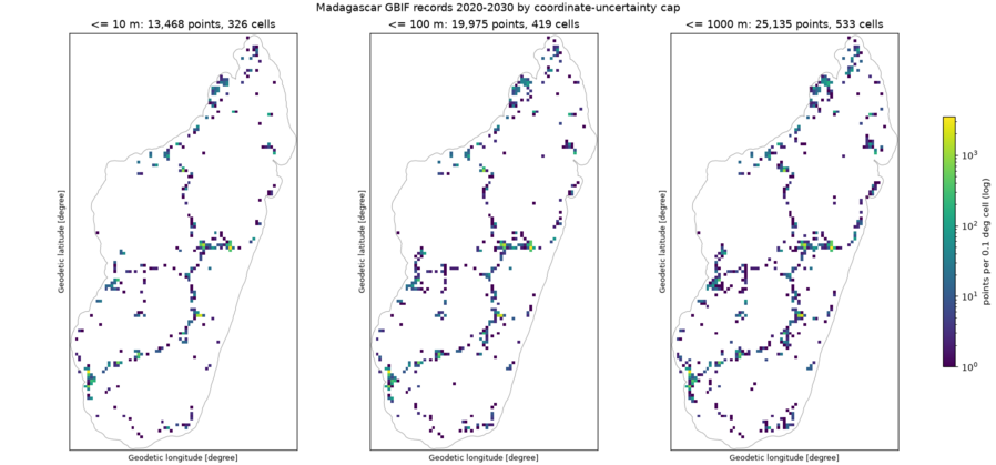
That's not to say the data isn't useful, but it's also not the magic bullet one might assume it would be in the data-sparse areas. I'll be interesting to see how this map changes once we add the eBird data.
I did some other cuts of the data too: rather than just trying to move to a global set of labels contributing to the map of a region, I took a look at how that would work with an expanding buffer, to try keep the labels somewhat local (e.g., 500km, 1000km, 2000km). Mostly this doesn't look good for my normal two test areas, UK and Madagascar, as they're surrounded by water, particularly Madagascar. Going by latitude band instead does help, but mostly I suspect because for Madagascar that pulls in northern Australia, where you once again get into people have more free time and mobile phone access to contribute to things like iNaturalist. Nothing conclusive as a result, but it's interesting to start wondering about these things, as pure global runs will be quite expensive in compute.
More robust analysis of maps
Whilst I was in eBird data limbo, I invested time in improving how I validate our map runs. Like with any iterative research project, when I started I did something minimal so that I had some way of getting a sense of how well I was doing without spending a lot of time on it when we didn't know if the project has legs. However, I also knew that as we grew what we were doing wasn't good enough: in Madagascar and Minas Gerais we were outscoring the related work despite being poorer visually, driven by the scarcity of occurrences somewhat, but also by poor method on my behalf.
My high-school maths teacher opened up the final year with the statement that she didn't like probability maths, and so we'd be skipping that module, and whilst I agree with their reasoning, it has meant I'm always slightly on the back foot with statistics and analysis, and so I had to play catch up as I upgraded the evaluation for what is building a statistical product. I know understand k-fold cross validation (also random-cross validation), and more about spatial cross-validation (which I shared a bunch of papers Aneesh Naik had pointed me at last week - the opening of this paper makes for a good review of why you'd want either method).
By the end of the week I implemented the k-fold random-CV, and it started to highlight the weaknesses of my approach in data-deprived areas against the other metrics, which is good, as the results it gave before were just clearly biased on the samples I was using. One particularly silly flaw was that as the pipeline evolved to add more filtering of points, the separation of training data was happening downstream of those, which is clearly bad practice also. Amusingly though, fixing this caused all validation scores to drop - because my filtering of GBIF data was actually cleaning up errors in the original data - so all methods performed better if you do that. Still, I was benefitting more because this influenced my training data - so it's good to get all this fixed.
The spatial-CV I'm currently still waiting on to run for the regions of interest. The challenge with spatial-CV is that the point density, despite the thinning work I did last week, is still very un-uniform across regions, and so I can't just do a straight regular grid for this, and I'm evaluation the CAST R package to automatically generate cells with equal occurrence density.
Wood pigeons are a worse case scenario
As a fun point to wrap all this up for these weeknotes, I did discover that, in the UK at least, the Wood Pigeon is empirically (using our new new random-CV testing) the enemy of my software :)
| All species UK | Wood pigeon UK | |
|---|---|---|
| Ours | 73.9% | 21.9% |
| Jung L2 errata | 62.8% | 55.4% |
| Lumbierres/Copernicus | 61.6% | 63.3% |
So what's going on here? Well, if you look at the IUCN Red List habitat data for the Wood Pigeon, it lists many kinds of artificial habitat, but not urban. However, in the UK I think I've mostly only ever seen them in urban environments - we had a pair that nested in our back garden for many years. From this I'd argue that they're misclassified. This is then compounded by most occurrences being recorded by people in urban areas. Our pipeline then throws all that data away, as it tries to clean up the data, and isn't something the other methods do, so they score much higher than we do. It's a sort of perfect storm of our various datasources.
One thing that helps Lumbierres et al here is that they allow multiple mappings from the Copernicus Land Cover Map they use as their base layer to IUCN habitat classes, and indeed map "built-up" to both Urban and Rural Garden. In theory, this is wrong based on the definition of rural garden being a small farmsted according to the IUCN guidelines, but it does reflect the data, and so I think leads to a better habitat map that captures the IUCN habitat classes as used rather than as defined. This is something I'm keen to capture, and now I realise my OSM filtering stages might need to be slightly more forgiving, as I've based them on following the IUCN habitat class definitions quite closely.
Part II Students
I mentioned last week that I have one final year undergrad project to supervise this coming academic year, but now it looks like I'll have a second one! The first one is looking at improving dynamic resource adaptation in my declarative geospatial library Yirgacheffe, and the second is working with the aforementioned GPS accuracy issues, a topic suggested by Aneesh when the student in question expressed an interest in doing something related to Tessera, and it suits me as it's a topic clearly close to what I'm working on.
For readers not in Cambridge: the undergrad course here is three years: part I-A (one A - aka first year), part I-B (one B - aka second year), and part II (two - aka third year). As someone who was never a student here this still causes me to pause to think every time I bump into this. My understanding is that it's a historical quirk that has never been updated, and I just felt that given I'm going to be saying "part II projects" a lot in the coming months I should just get this out the way.
This coming week
- Finish of the spatial-CV integration
- Review the impact of the eBird data on data-deprived areas like Madagascar and Minas Gerais before we move on to global labels.
- Make sure the part-II project students are unblocked.
Tags: weeknotes