Processing geospatial data at render time on GPUs using Shaders

24 Jul 2022

Tags: 4C, geospatial, geotiff, gpu, metal, shaders, swift

I recently wrote up about how I was playing around visualising some geospatial data around forest loss at the Cambridge Centre for Carbon Credits (4C), and in particular how I was pre-processing the Hansen lossyear dataset offline so that I could generate map tiles from that. In this article I’m going to show how I ditched that pre-processing stage thanks to using GPU shaders to let me do the visualisation transformation at view time instead, saving me a lot of bandwidth and data storage.

Whilst the 4C work was in javascript and webGL, I recently wanted to give a live-coding demo of this idea in a talk I was giving, which was easier (for me) to pull together in Swift and Metal (Apple’s languages for writing CPU and GPU code respectively), so all the examples here will be using that code, but conceptually all this works roughly the same whether you’re using Javascript with WebGL, Swift with Metal, or C++ and CUDA. This isn’t going to be a tutorial on how to use Swift and Metal, rather just a fun simple intro to shaders, but if you do want to learn more about using Metal for GPU Compute, I can recommend this series of posts by Eugene Bokhan.

The code for my stand alone demo can be found over on github. If you have a Mac and Xcode you can play along just by tweaking the Lossyear.metal file and re-running it.

So a quick recap of the context: I have these large GeoTIFF files from the Global Forest Watch team that show where tree loss occurs over the last 21 years. The data is encoded in these TIFF files, with pixels in the image representing a section of the planet’s surface, with each pixel having a value of 0 for no loss, or the number 1 through 21 to indicate the first year when the forest in that pixel was first lost (if at all). Although technically a valid TIFF image, clearly the image contains raw data rather than visual information, so in my last post I talked about how I was processing this single GeoTIFF to make 21 other GeoTIFFs, one per year, that showed the accumulative loss until the respective year encoded for display - black for no loss, white for loss before the file’s respective year - and you can then swap out the right tiff in response to a slider in our website to let people interact with the data. Whilst this solution worked, it was clearly somewhat storage and bandwidth heavy.

The inspiration for doing the year processing client side came from two things. Firstly, I looked into speeding up the script I had for taking all the Hansen tiles I was interested in and splitting them out by getting the GPU to help: I’m processing pixel data, and this to my mind is something GPUs should be good at. At the same time my 4C college Sadiq, who didn’t like the monochromatic tiles I was outputting, introduced a webGL shader in the 4C visualisation tool that would re-colour the tiles I generated when displayed - essentially he used the GPU to process my files on the fly as they were rendered to screen.

Seeing both of these it dawned on me that if we were using the GPU on the browser to re-colour things, couldn’t I just take my existing GPU code that I had for processing the raw Hansen data on the server side and build something that used a lot less storage and bandwidth? A simple idea, and it works a treat. So this is a little look at how it works.

So let’s start with a look at a what a shader is at its most basic. A shader is a small bit of code that has a pixel centric view of the world. You have one or more input images of the same size, and shader will take the same corresponding input pixel from each image, do a bit of calculation work, and then generate a new pixel value for a destination image in that same corresponding position. What makes shaders so powerful is that a GPU can run potentially thousands of copies of this code in parallel at the same time, whereas on the CPU you’d be able to process a small handful at best.

Best analogy I’ve seen (from The Book of Shaders, more on that below) is a CPU is like writing out by hand, and GPU is like a letterpress: writing by hand is slower, but very flexible; a letterpress takes a while to set up, but once done every letter on the page appears at once.

GPUs can achieve this massive parallelism because the functions within shaders are kept generally quite computationally simple. If you need to do something complex to your pixels, the CPU may still be your best bet (e.g., time series analysis of pixels over a series of images). The GPU has another downside in that soften it needs the data to be copied to a separate memory area, and moving data around a computer is a low slower than a CPU can do work, so for small numbers of pixels you may find the that the CPU is still faster.

But, in my little test application, we hit the perfect shader use point: we have a computationally simple problem, and map data tends to get big quickly. Anyway, enough waffle, let’s have a quick look at a simple shader in action

Lets start with the most simple shader - one that takes a pixel and returns the same pixel:

float4 my_shader(float4 pixel, float year) {
    return pixel;
}

Here you get to see the template of our shader - it’s a simple function that takes in a single pixel, and the year we’re interested in viewing, and returns a new pixel value. In this instance we’re not modifying the data, so we ingore the year that is passed in, and what you see looks like a blank image in and a blank image out. However, the image only looks blank to us humans, because the TIFF file is storing the loss year as a value between 0 and 21, but in the TIFF world 0 is black and 255 is white, and so 21 is still pretty close to black. So if I scale up the pixel by multiplying it by a large number, you can see the raw values emerge (I’ve scaled it by an overly large number so you can see all the data effectively):

float4 my_shader(float4 pixel, float year) {
    return pixel * 200;
}

So, as you can see, there is some data in there as promised (this is the same as when in my last post I scaled up the data using Photoshop).

Now, in the shader a pixel is just a struct with 4 floating point numbers in it that go from 0.0 to 1.0, one each for Red, Green, and Blue visible channels, and one for the transparency, known as alpha. We can set the individual channels if we want like this:

float4 my_shader(float4 pixel, float year) {
    return float4(1.0, 0.4, 0.4, 1.0);
}

Not a very useful shader, as just ignored the input pixel value, and made everything pink, but you can see how we can influence the output more than just math on what was passed to us.

So, if we now combine this with the year parameter passed in, and say that value is set to map to the year 2021, then we can see how we can create an overlay texture to put on a map, by returning pink where the loss event happened before the year in interest, and emitting a transparent pixel in the places where either there was no loss or it is yet to occur:

float4 my_shader(float4 pixel, float year) {
    if ((pixel.r > 0.0) and (pixel.r < year)) {
        return float4(1.0, 0.4, 0.4, 1.0);
    } else {
        return float4(0.0, 0.0, 0.0, 0.0);
    };
}

All of this seems quite simple, and it is. The thing that makes a GPU fast is that is does a simple thing many, many times, so on my MacBook Pro on which I write this it can process nearly 2000 pixels at once, and if you get the current top of the line Apple Silicon chip it’s pushing over 8000 pixels at once.

It’s worth noting that in the last example we have some control flow, with two possible branches being taken. Earlier I made a comment that you don’t want complex algorithms in a shader, and that’s because every cell in a GPU (at least to my understanding) has to execute the same instructions, and it’s just selective about which results which cells store. So every time you add a branch you slow down your code more than you would on a CPU where you just take the branch of interest (kinda, speculative execution on CPUs makes a mockery of that simplification). Thus you really do want to be selective about what logic you put in your shaders: as a crude example, if you had two processing algorithms to pick from say, you’d not want to put both in one shader and pass in a parameter to select the algorithm, you’d want two shaders and to pick the right one before you process the image.

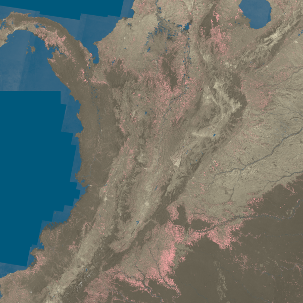
As another example, here’s the shader I use to generate the landscape background for my little application:

float4 landsat_shader(float4 pixel) {
    return float4(
      (pixel.r * 2) + (pixel.a * 2 * 0.8),
      (pixel.r * 1.8) + (((pixel.a * 2 * 0.7)
        + (pixel.b * 0.5)) * (1.0 - pixel.g)),
      (pixel.r * 2) + (pixel.a * 2 * 0.5),
      1.0
    );
}

The input to this one is a subset of the NASA Landsat data provided by Hansen. It encodes different wavelenths in the four pixel channels:

Red: is red visible light, which is good for visible feature identification.
Green: Near infrared, which is good for spotting healthy vegetation.
Blue: Short Wave Infrared band I, good for spotting wet earch and differentiating rocks and soil.
Alpha: Short Wave Infrared band II, similar to the above.

You can read in more detail about the different Landsat bands here, including the other channels that Hansen don’t include. What I do in the above shader is try to make an artificial colouring that looks a bit like we’d expect a map of forest areas to do so, and emphasis vegetation, as you want to know if there’s no forest loss whether that’s because there’s been no loss, or there was no forest to start with.

For completeness, here’s the last shader I wrote, which takes the mask layer Hansen have that delineates between no data, water, and land, and I use it to generate an overlay for the Landsat map to mask off the water areas. Again, the original values for the three layers are such that they all appear different shades of near black when we try to view the original image, but a little filtering reveals the data within:

float4 mask_shader(float4 px) {
    if ((px.r > 0.0) && (px.r < (1.0/2000))) {
        return float4(0.0, 0.0, 0.0, 0.0);
    } else {
        return float4(0.0, 0.1, 0.2, 0.5);
    };
}

I then combine my three images using another set of built in combination shaders to CoreImage, the image library in Apple’s platforms, to output the result:

In theory I could also just write a single shader to do all of the above, because as mentioned before a shader can take pixels from multiple images, but for the purposes of the talk I was giving it was nice to keep things simple like this.

Hopefully that gives you an idea of how shaders work and how they let you do simple processing on not just images, but also raw science data and let you visualise it on the fly as it’s being drawn to the screen. You can also obviously use the same code to write to images - all the example images with my code snippets were just saved out of my little test app using the exact same code as I used to draw on screen in my app.

The thing I didn’t show you in this post, which is also somewhat of a pain when using webGL or Metal like this (I’ve not tried CUDA, so can’t comment) is the setup work required to get to the point you’re using a shader, which can be quite laborious if you’re not using a framework to hide it all away for you.

If you want to learn more about shaders in detail, then I can recommend The Book of Shaders, which is a very accessible guide that goes into a lot more detail than I will in this post. They even have little interactive bits of webGL where you can play with shader code in browser and you can see the impact in real time, and examples where you can tie the shader to inputs like time and cursor position - a really fun way to get to learn more.