Weeknotes: 19th October 2026
Pondering test data selection
Last week I talked about two strands of work on the habitat map work: improving the robustness of my validation approach, and integrating eBird into my occurrence data alongside that from GBIF. I spent some time wrapping up those bits, and am now quite pleased with where we are.
One interesting thing that fell out of all this was there's a subtle but interesting decision point as to when in a pipeline to split out your test data from your training data. Looking back at what I was doing previously and comparing that with other published work that validates itself in a similar way, I suspect that I'm not alone in this error because it's a slightly easy trap to fall into. Let me explain.
In this pipeline, like many other pipelines, I'm taking some samples from the real world, cleaning them up to try to remove problems with the real world source data, and then applying that to a statistical model (in this case, it's a machine learning model, but that's still just a very fancy statistical model in my book). At some point in pipeline you want to take some of your input data and use that for validation, and the question is when do you do that? You could take it right at the start, so you're not biasing the results by being selective, or you could take it somewhere later once you've done some quality checks on the data to remove obvious outliers - we work with species occurrence data on this project, and not every occurrence record is correct, as it can be hard to tell what species you're looking at sometimes, or your GPS record could be wrong, etc. If you're testing your results against existing work, then doing this will improve the scores for both works, so this seems fine.
However, at some point, your improvements are non-standard (I'm talking about this in a research context, not an engineering context, so at some point your new method comes into play), and even though you think you're doing good to clean up the data, it's really your own method you're testing at this point, and so you're starting to bias the sample data in your favour. For example, as I described last week, I use OpenStreetMap to help clear up occurrence data, and the numbers show that doing this improves the validation score for both my habitat map and for the two other maps I'm comparing against, but it improves my scores a lot more than the others, so whilst I think I've done the right thing here, I feel I should choose before I do any custom filtering. But perhaps that means the other maps were trained on bad data, so I should be doing this filtering? It's all a bit murky.
I think the main guiding principle here is to be transparent about how one is doing it. Reading the other papers I suspect they've not considered this as much - which is fine, as they weren't trying to contrast their work with others, being pioneers in the space, but it is something I think I need to be cognisant of. For now, I think the most defensible thing I can do is draw the line after doing existing published occurrence cleaning techniques from other papers, such as Boitani et al 2011 (not that I believe that to be a gold standard, but it is an agreed upon standard), and then my own cleaning I will defer after the training split, or if I do chose to do more filtering I should publish the impact in addition to the cleaning that is agreed upon by others.
Ultimately, why are we validating? It's not that I want to be best so I can win a race, it's because I want to try and improve the state of the art, and comparative validation is the only way I can track if I'm helping the world of ecology or not. I do believe our approach has promise, but I need to try and convince myself that what I'm going to share with people is better as much as I need to demonstrate it to others. It's easy to pick numbers that paint us in a fair light, but the point here is to try do something to help save the planet, and so I want the assessment to be properly critical of my work so that others can build upon it in confidence.
Urban spread
As noted last week, adding the eBird data wasn't the automatic win I had naively assumed it would be. In Madagascar whilst there are four times as many occurrences in the eBird data as there are in GBIF, it actually doesn't improve our area coverage significantly: most of the samples are taken at places already covered by other datasets. However, that wasn't true for my other test region, the Brazilian state of Minas Gerais: eBird data did actually expand area coverage by a meaningful amount, and so I generated an updated habitat map for that region.
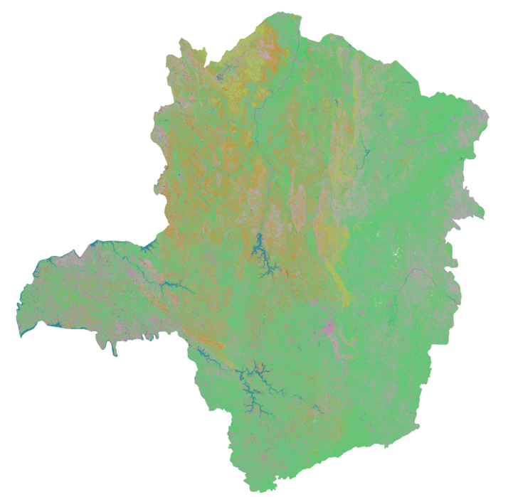
The map is looking a lot better than it did the last time I generated one, but is still quite flawed, for many reasons. Some of those I hope will be tackled as we go from regional maps to global maps, but there is one common issue that I see in all my maps, regardless of whether they're data-rich or data-deprived (it just is worse in data-deprived regions), which is the maps falsely showing urban habitats where we don't expect to find them. You can see this in the dark pink pixels in the western bit that sticks out to the side (Triângulo Mineiro), but it's also a problem in the UK where we have plenty of data, so what's going on?
The root cause here is that we have two real problems, which are then compounded by a third:
- Most occurrence data for species, particularly in data-deprived areas, is taken in "urban" environments.
- In the IUCN habitat classification system v3.1 there is just one habitat class for urban (14.5).
Urban unfortunately isn't one type of habitat really: it covers buildings, and parks, and gardens, and roads; it covers high density city centres and low density villages. So we end up in a situation where most of our data isn't from natural habitats, and worse it is from the non-natural similar looking bits of so called urban environments. This means even in the data-rich UK I see urban polluting areas where it shouldn't in my habitat map: tops of mountains are rocky reflective areas, which look a bit like buildings so get classified as urban; rocks on the shore lines, perhaps are a little bit like roads, come out as urban; hedges between fields in farmland, well most hedges in my sample are in gardens so yes, urban again; grassy pasture that's been well cropped, looks a bit like a park, must be urban.
Just to give you an example, here's some UK farmland from a version of my map before I started to try correct for this:
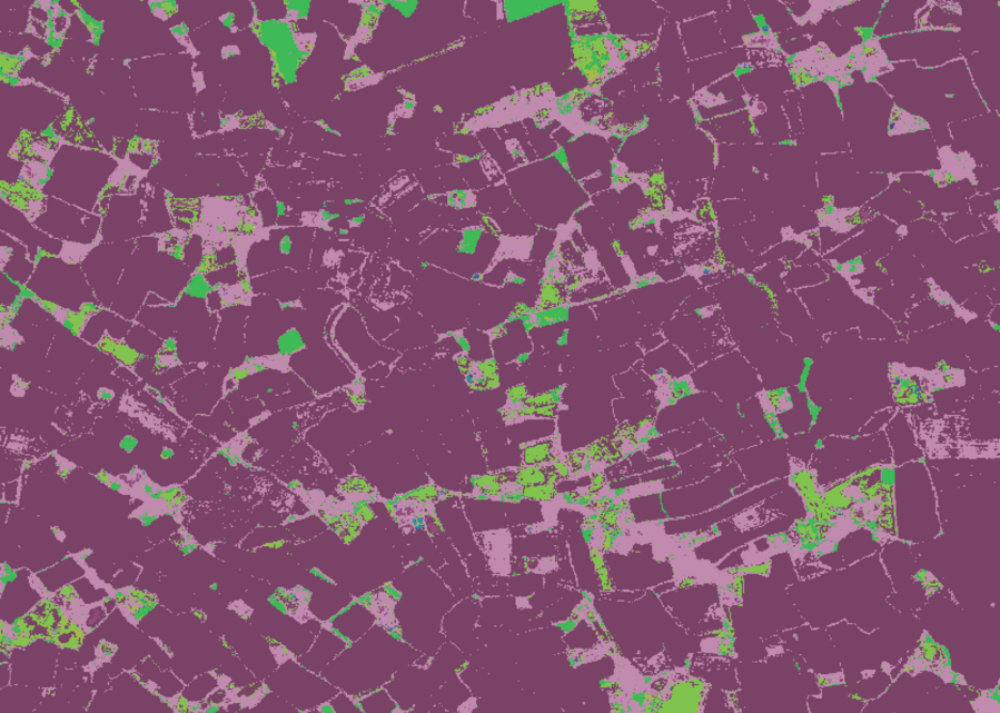
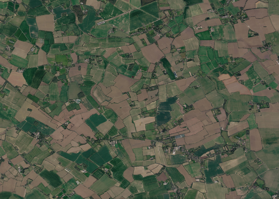 PredictedSatellite
The dark pink is where we predict arable farmland, light pink is where we predict urban, the light green is predicted grassland, and the dark green forest. In the UK 42% of my occurrences are urban, 20% forest, 7.5% arable, and 7.5% grassland. Given the bias in the data it's not a surprise that we end up thinking everything is its artificial variant. In Minas Gerais 38% of labels are urban also, sitting just ahead of moist lowland forest at 35%, but then we have a big gap to degraded former forest at 12%.
So now we come to the third problem: biases in data like this are nothing new, and there are methods to deal with this, just I'm not using them as I'm pretty new to this machine learning/statistical modelling world. Thankfully I have smart colleagues I can turn to for assistance! I had discussions with both Sadiq Jaffer and Aneesh Naik, and they pointed out that the classifier I've been using for my map inference stage isn't up to snuff, and that I need to up my game.
Until now I've just been following the Tessera 101 example Anil Madhavapeddy put together for me a while ago. Being a simple tutorial it just used a simple classifier for the map inference stage, a k-nearest neighbours strategy, which for each pixel you're trying to guess, finds the labelled pixels with the nearest value to your guessing pixel in the Tessera embedding space, pick the top k (say k=5, you take the top 5) labelled pixels that are closest, and take the most common label. I like this, because as a machine learning newbie it's easy to understand, but it's also easy to see that if you have a biased dataset where say most hedges are labelled in urban gardens, then when we see hedges in fields we'll end up saying it's urban.
To solve this there are better classifiers, such as linear classifiers, and then balanced classifiers within those, that try to do a better job of not letting a single group of labels win just based on weight of numbers. Thus I've spent a day skilling up on linear classifiers. I have just about got my head around them, and initial results certainly show this is helping, but before I got too far with that I hit another issue...
There probably aren't mangrove forests in Scotland (yet)
Whilst using a linear classifier did look good, trying to use a balanced linear classifier made some really bad maps, and so I needed to look into why. In theory a balanced classifier tries to weight the different classes based on how many samples they have, so the fact we have more variety in urban pixels isn't as influential as the fewer pixels we have for say rocky areas. My usual test case for this is Skye, where the Black Cuillin mountain tops come out as urban with Tessera v1.1 (as an aside, Tessera v2 does fix this, but I'm stuck on v1.1 as Tessera v2 doesn't have global coverage yet).
Here we can see the difference going from the kNN classifier to the linear classifier:
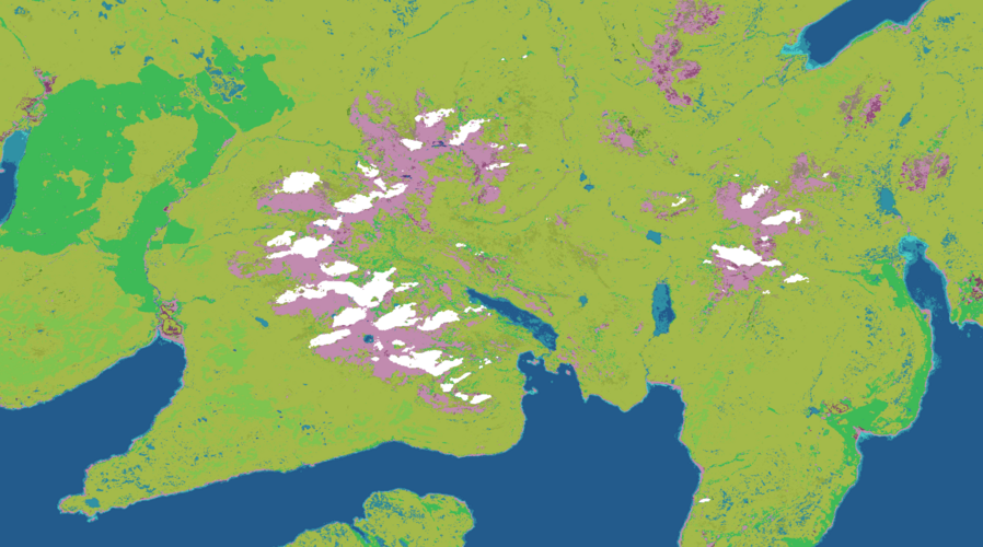
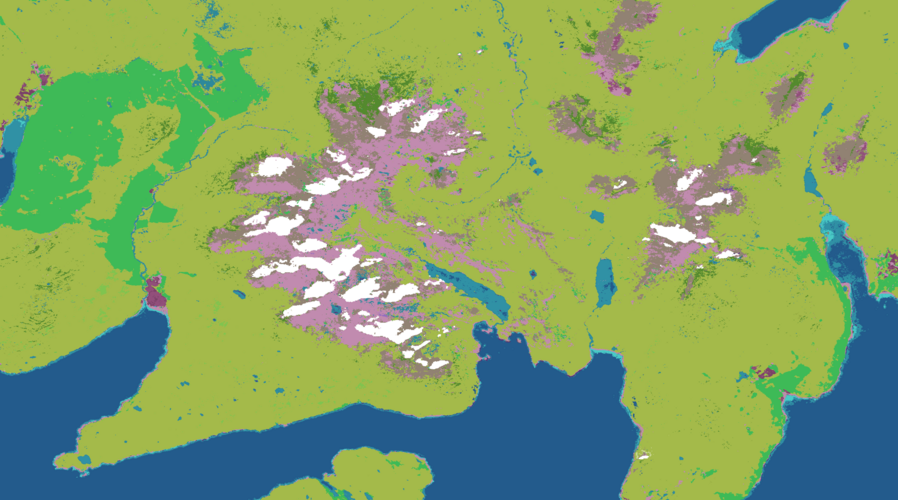 kNN classifierlinear classifier
You can see that we go from that light pink urban area to a mix of grey and pink - so somewhat rocky, but not perfect. The white areas are areas where Tessera doesn't have enough data due to somewhat persistent cloud coverage across 2025 btw :) So now if we try to balance the classes (admittedly somewhat naively):
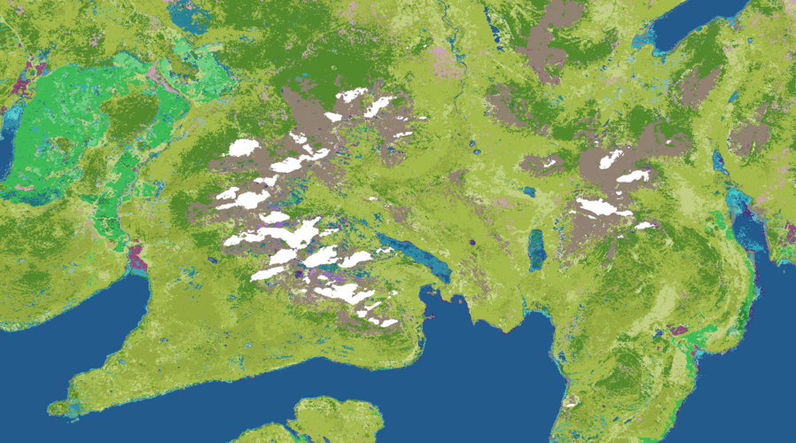 linear classifierbalanced linear classifier
The mountain tops are now rocky, which is great, but what's happening to the rest of Skye? We suddenly have a lot more variety in the terrain, including "Forest - subtropical/tropical mangrove vegetation above high tide level" 🤦 I'll admit, I've not been to Skye for a few years now, being there for my sister's wedding in 2018, but I don't think it'll have changed that much that quickly.
This time, unlike last week, it's not the Woodpigeon that is to blame for my woes, but rather birds like the Grey Heron and Little Egret. In my pipeline we see occurrences of those species, take from the IUCN Redlist the habitats they are known to prefer, and then filter each occurrence by what Open Street Map says is there. Unfortunately whilst the IUCN habitat specification is crude for urban areas, it is quite specific around forests, grasslands, and shrublands, breaking each down to classification based on rough latitude bands: boreal, temperate, subtropical, etc. OSM on the other hand is crude, and says "forest". Birds like the Grey Heron and Little Egret get their food by fishing, which means coastal areas or river areas in the UK, but in other parts of the world they can do that in Mangrove forests, so the only type of forest that they like isn't to be found in the UK (at least naturally). But when we filter their habitats based on OSM, the best we can say is "someone saw a heron in a forest", and the only forest a heron likes is mangrove, so this must be a mangrove spot! 🤦
Now, before, in my kNN classifier there were so few of these it didn't matter that this mistake happened. But if we artificially balance the different classes we have, suddenly all these little mistakes that get through my filtering have their importance made equal to every other class, and bam, we have mangrove forests on Skye :)
This relates to a problem I'd discussed with my colleagues Alison Eyres and Shane Weiss a while back but hadn't really actioned because it wasn't a problem, but now it is I went back to Ali and we discussed how we might bring in another data source to try and make up for the fact that our current pipeline can't tell that certain types of forest are restricted spatially due to climatic conditions. In the end we've opted for using a combination of biome data from the RESOLVE Ecoregions dataset and the Köppen-Geiger dataset - both of which are used in the production of the Jung et al habitat map. Unfortunately neither is sufficient alone to try and let me filter occurrences, so I have to use the former, and where it is deficient the latter. There are also cases where they disagree, which is unfortunate, but I think at broad strokes that'll help pin things down.
But that's where I got to before the week closed, so we'll see how this goes the coming week. Either way, moving off a kNN classifier to something more nuanced is a good move, and actually aligns with the statistical model used in the Lumbierres et al paper that I've been inspired by, so I'm pleased with the input from all my colleagues this week.
Basically this last two weeks, between the classifier work and the validation work, I've had to learn a lot about an area I wading into somewhat uneducated, and so it's been slow in terms of output, but I feel I'm getting a lot out of it, and feel grateful (as ever) to be surrounded with such smart people.
Mapping urban wild animals
My friend Adrian sent me a link to mapping wild animals in NYC with open and crowdsourced data. Clearly given the urban bias in data we should be able to do something similar for Liverpool, just not with my habitat map as a basis, as it just says Liverpool is "urban" and so makes for a boring map.
I live just outside Liverpool, and being a coastal city, the range of wildlife we have here is quite impressive, it feels more so than when I lived just outside Cambridge. I regularly see the aforementioned Little Egrets and Grey Herons whilst cycling between here and Liverpool, we know that there are porpoises in the Mersey, etc. One of the unexpected side effects of moving has been just how much more wildlife I see on a regular basis now that I'm not living in an area dominated by arable farmland. That said, I do miss the Muntjac Deer and Badgers that would regularly visit our garden back in Cambridgeshire - just they would visit at night mostly, so perhaps that's the main difference: there's animals all around if you know where and when to look.
Yirgacheffe
I was meant to attend FOSS4G:UK last week, presenting a talk about Yirgacheffe, but had to pull out due to being unwell at the last minute, which was disappointing. One thing I've failed to do is solicit more feedback on Yirgacheffe's approach from the GIS open source community and I was hoping this would be a good point to do that, and unfortunately missed out.
Still, I did a small update release to Yirgacheffe, adding the ability to create vector layers directly from WKT (Well Known Text) format, and added support for trig operations like numpy.
This does remind me that I need to do an API tidy up in 3.0 to deduplicate how you call things like this. I'm an old Python programmer, and did a lot of Django in the day, and so am very used to method chaining, which means I wrote Yirgacheffe originally like:
result = my_layer.()()()
But at some point my colleague Patrick Ferris pointed out that this isn't the idiom used by the data-science libraries my target audience were used to. In numpy you'd write:
cleaned = np.()
trigged = np.()
result = np.()
And so around the run up to 2.0 (which took about a year) I added support for that too, so with Yirgacheffe you can replace np with yg and you're good to go. But I didn't remove the more object-orientated version, as I quite like that way. But over time, as I've added more and more support for different operators, this is now becoming somewhat of a maintenance pain, particularly as I end up duplicating a lot of test cases for both formats.
Either I need to look into code generation so that one is automatically derived from the other in a way that is robust and trustworthy, or I probably need to switch to the numpy style and drop the OO style in 3.0.
Not the end of the world, just an example of the tedium of API design :)
This week
- HABITAT MAPS IT NEVER ENDS. I enjoy the work, I just feel I need a better way to write this bullet point each week.
- The CFP deadline for Alpaca Festival is coming up fast, so I had a chat with Patrick about where I'd got to with my browser port of my OCaml graphics library Claudius, as I really want to do a functional-generative-art-in-OCaml talk or workshop. I have two weeks to try to make that a thing.
Tags: weeknotes, yirgacheffe, habitat mapping, tessera